Motivation

This post is motivated by a fantastic video (by 3blue1brown) regarding complex Fourier series. Here I want to give a brief overview of how to do the Fourier transform for a complex function and also how to implement it in Julia with few lines of code. Furthermore, a few different ways to generate a parametric curve to use as an input for our program.

Before we dive in, I want to emphasize how interesting the outcome of this work is. Basically, given any 2D shape, we want to find \(n\) fixed length vectors, each rotating at a constant speed such that if we add them together, they draw the input shape. This is an example with 600 vectors, drawing the word “hello”:

Complex Functions

Let’s think of a complex function \(\, f(t)\) which takes an input between 0 and 1 and outputs a complex number. We can visualize the output of this function on a 2D plane with x-axis being the real component and the y-axis being the imaginary component.

Complex numbers provide an elegant way to store the 2D coordinates with the additional benefit that \(e ^ {it}\) walks around a circle with a constant speed of one unit per second. For convenience, we can work with \(e ^ {2 \pi it}\) instead, which loops exactly once around the circle as \(t\) goes from \(0\) to \(1\), as shown below.

Note that \(e ^ {2 * 2 \pi it}\) goes twice as fast and \(2 e ^ {2 \pi it}\) walks around a circle twice larger. Now, by combining different terms you can create interesting shapes. For example:

Here is the code in Julia to generate this animation:

using Plots
using Interact
using JSON
gr()

pw = (t, x) -> ℯ ^ (x * im * 2π * t)
func = t -> (0.1 - 0.5im) * pw(+1, t) +
            (1.0 + 0.5im) * pw(-1, t) +
            (0.0 + 0.5im) * pw(+2, t) +
            (0.5 + 1.0im) * pw(-2, t) +
            (1.0 - 0.5im) * pw(+3, t) +
            (0.3 + 0.5im) * pw(-3, t)

anim = Animation()
xs, ys = [], []

for i in 0:0.01:1
    plot([], [], legend=nothing, aspect_ratio=:equal, xlim=[-5, 5], ylim=[-5, 5], widen=true, framestyle = :origin)
    x = real(func(i))
    y = imag(func(i))
    annotate!(x * 1.2, y * 1.2, text("$i", :center, 10))
    append!(xs, x)
    append!(ys, y)
    plot!(xs, ys)
    quiver!([0], [0], quiver = ([x], [y]))
    frame(anim)
end

gif(anim, "complex.gif", fps = 15)

Complex Fourier Transform

Now, how would you combine these exponential terms to draw a given shape such as a bird, heart, handwriting, etc.? Also, is it always feasible to do so? Basically, given a function \(\, f(t)\) can you always represent it in terms of a summation of these exponential terms with some complex coefficients? \[\begin{equation} \begin{aligned} f(t) &= \cdots + \, c_{\color{magenta}{-2}} \, e^{\color{magenta}{-2} \, 2\pi i t} + \, c_{\color{magenta}{-1}} \, e^{\color{magenta}{-1} \, 2\pi i t} + \, c_{\color{magenta}{0}} \, e^{\color{magenta}{0} \, 2\pi i t} + \, c_{\color{magenta}{1}} \, e^{\color{magenta}{1} \, 2\pi i t} + \, c_{\color{magenta}{2}} \, e^{\color{magenta}{2} \, 2\pi i t} + \cdots \\ \end{aligned} \end{equation}\]

Joseph Fourier in the 1800s proved that it’s always possible (under some basic conditions ¹). Let’s look at a brief overview of how to do it. Suppose the transform exists and let’s try to extract the coefficients \(c_i\). Take an integral from \(0\) to \(1\) on both sides. Note that for any exponential term, if the power is a multiple of \(2 \pi t\) and non-zero, as \(t\) varies from \(0\) to \(1\), it loops around a circle once, twice, thrice, or more. but it is important that it does full loops. so, the average of all these points (aka the integral from \(0\) to \(1\)) will be zero. The only term that remains non-zero is \(c_0\). \[\begin{equation} \begin{aligned} \int_{0}^{1} f(t)\,dt & = \int_{0}^{1} \left[ \, \cdots + \, c_{\color{magenta}{-2}} \, e^{\color{magenta}{-2} \, 2\pi i t} + \, c_{\color{magenta}{-1}} \, e^{\color{magenta}{-1} \, 2\pi i t} + \, c_{\color{magenta}{0}} \, e^{\color{magenta}{0} \, 2\pi i t} + \, c_{\color{magenta}{1}} \, e^{\color{magenta}{1} \, 2\pi i t} + \, c_{\color{magenta}{2}} \, e^{\color{magenta}{2} \, 2\pi i t} + \cdots \right] \,dt \\ & = \, \, \cdots \, + \, \int_{0}^{1} c_{\color{magenta}{-2}} \, e^{\color{magenta}{-2} \, 2\pi i t} dt + \, \int_{0}^{1} c_{\color{magenta}{-1}} \, e^{\color{magenta}{-1} \, 2\pi i t} dt + \, \int_{0}^{1} c_{\color{magenta}{0}} \, e^{\color{magenta}{0} \, 2\pi i t} dt + \, \int_{0}^{1} c_{\color{magenta}{1}} \, e^{\color{magenta}{1} \, 2\pi i t} dt + \, \int_{0}^{1} c_{\color{magenta}{2}} \, e^{\color{magenta}{2} \, 2\pi i t} dt \, + \, \cdots \\ & = \, \, \cdots \, + \, 0 + 0 + c_{\color{magenta}{0}} + 0 + 0 \, + \cdots \\ & = c_{\color{magenta}{0}} \end{aligned} \end{equation}\]

This is nice because it allows us to calculate \(c_0\) by integrating over \(\, f(t)\) from \(0\) to \(1\). Now, we can use a clever trick to calculate any \(c_i\) in the series. For example to calculate \(c_2\), multiply both sides by \(e ^ {-2 * 2πit}\) and then take the integral. This time, all terms become zero except \(c_2\). \[\begin{equation} \begin{aligned} \int_{0}^{1} (e^{\color{magenta}{-2} \, 2\pi i t}) \, f(t) \,dt & = \int_{0}^{1} \left[ \, \cdots + \, c_{\color{magenta}{-2}} \, e^{\color{magenta}{-4} \, 2\pi i t} + \, c_{\color{magenta}{-1}} \, e^{\color{magenta}{-3} \, 2\pi i t} + \, c_{\color{magenta}{0}} \, e^{\color{magenta}{-2} \, 2\pi i t} + \, c_{\color{magenta}{1}} \, e^{\color{magenta}{-1} \, 2\pi i t} + \, c_{\color{magenta}{2}} \, e^{\color{magenta}{0} \, 2\pi i t} + \cdots \right] \,dt \\ & = \, \, \cdots \, + \, \int_{0}^{1} c_{\color{magenta}{-2}} \, e^{\color{magenta}{-4} \, 2\pi i t} dt + \, \int_{0}^{1} c_{\color{magenta}{-1}} \, e^{\color{magenta}{-3} \, 2\pi i t} dt + \, \int_{0}^{1} c_{\color{magenta}{0}} \, e^{\color{magenta}{-2} \, 2\pi i t} dt + \, \int_{0}^{1} c_{\color{magenta}{1}} \, e^{\color{magenta}{-1} \, 2\pi i t} dt + \, \int_{0}^{1} c_{\color{magenta}{2}} \, e^{\color{magenta}{0} \, 2\pi i t} dt \, + \, \cdots \\ & = \, \, \cdots \, + \, 0 + 0 + 0 + 0 + c_{\color{magenta}{2}} \, + \cdots \\ & = c_{\color{magenta}{2}} \end{aligned} \end{equation}\]

So we can calculate each \(c_n\) using: \[\begin{equation} \begin{aligned} c_{\color{magenta}{n}} &= \int_{0}^{1} e^{\color{magenta}{-n} \, 2\pi i t} \, f(t) \,dt \end{aligned} \end{equation}\]

Which can be done using numerical integration:

# numerial integration
function c_n(f, n)
    dt = 1e-5
    return sum(f(t) * ℯ ^ (-n * 2π * im * t) * dt for t ∈ 0:dt:1)
end

Once we calculate all \(c_n\) terms for a given range of \(n\) (say from \(-10\) to \(+10\)), we have our fourier transform. Here is the full code (~50 lines):

using Plots; gr()
using Interact

# heart shape
func = t -> 20sin.(2π*t).^3 + (20cos(2π*t) - 7cos(2*2π*t) - 2cos(3*2π*t) - cos(4*2π*t)) * im

# numerial integration
function c_n(f, n)
    dt = 1e-5
    return sum([f(t) * ℯ ^ (-n*2π*im*t) * dt for t ∈ 0:dt:1])
end

function eval_term(c, x, i)
    return c[i] * ℯ ^ (i * 2π * im * x)
end

function sum_terms(c, x)
    return sum(eval_term(c, x, i) for i ∈ c_range)
end

n = 100
c_range = -5:5
t = range(0, 1, length = n)
c = Dict([ (i, c_n(func, i)) for i in c_range ])

comb = x -> sum_terms(c, x)
z = comb.(t)
x = real.(z)
y = imag.(z)

anim = Animation()
xs, ys = [], []

idx = sort(collect(c_range), lt=(x,y) -> abs(x) < abs(y))
evs = [(i -> eval_term(c, t[i], j)) for j in idx]

for i in 1:n
    # draw shape
    plot(xs, ys, legend=nothing, aspect_ratio=:equal, widen=true, framestyle = :origin, xlim=[-25, 25], ylim=[-30, 25])
    append!(xs, x[i])
    append!(ys, y[i])

    # draw vectors
    u = [real(a(i)) for a in evs]
    v = [imag(a(i)) for a in evs]
    xx, yy = [0.0], [0.0]
    for i ∈ 1:length(evs)-1
        append!(xx, xx[i] + u[i])
        append!(yy, yy[i] + v[i])
    end
    quiver!(xx, yy, quiver=(u, v))
    frame(anim)
end
gif(anim, "test.gif", fps=15)

¹ _{It is always possible if both \(f\) and its Fourier transform are absolutely integrable and \(f\) is continuous. (more details)}

Input

In order to test our code, we need the mathematical representation of a 2D shape as a parametric curve. Below are a few different ways I achieved the parametric curve.

Heart

I found this parametric representation of a heart shape on the internet.

x = 16 * sin(2π * t)^3
y = 19.5 * cos(2π * t) - 7.5 * cos(2 * 2π * t) - 3 * cos(3 * 2π * t) - 1.5 * cos(4 * 2π * t)

Here are the Fourier representations with [6, 20, 100] vectors:

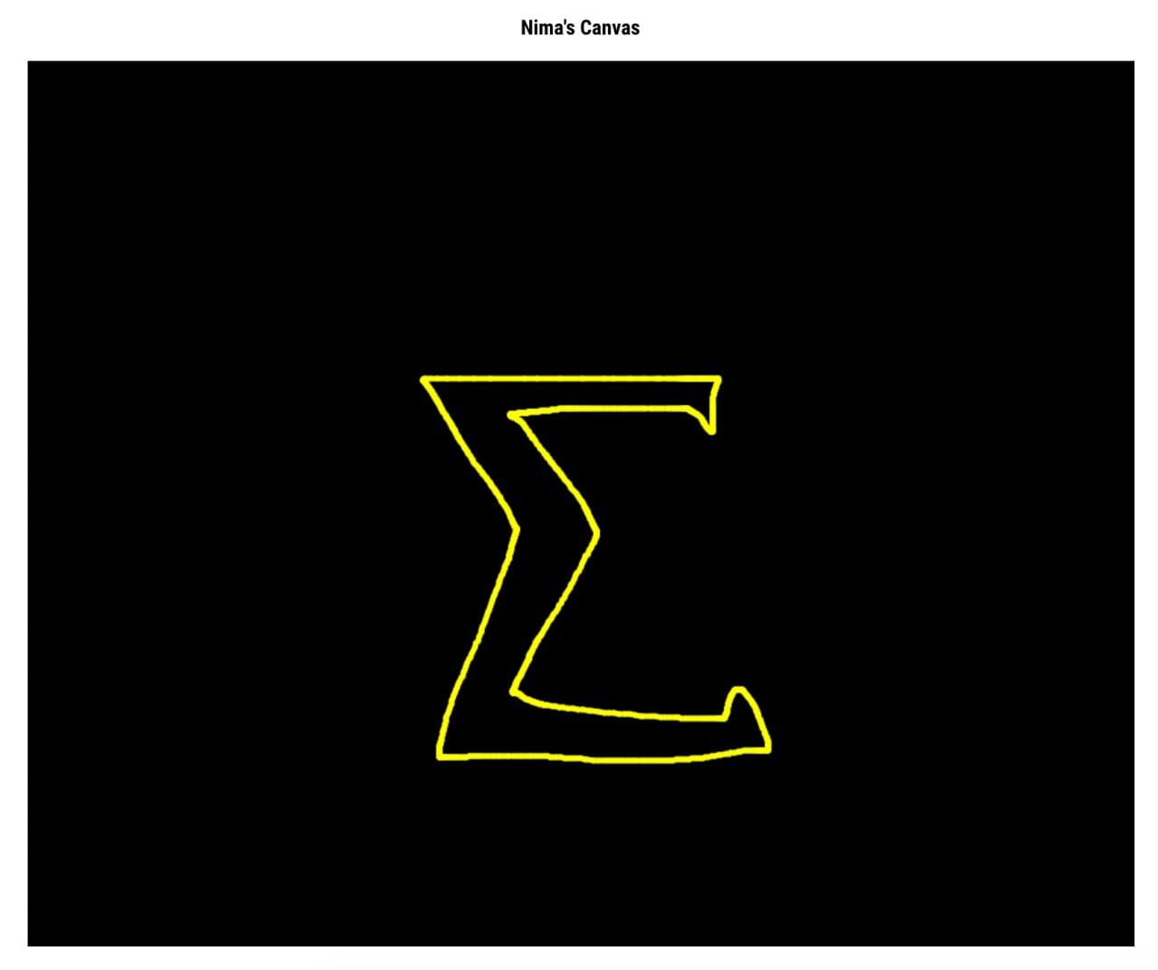
Sigma

I wrote a quick NodeJS app where you can draw a shape, and it gives you an array of points. (connecting each point to the next point results in the shape we want to draw). An example drawing:

Then we need to convert the list of points to a parametric curve. This can be done fairly easily as well:

function interpol(p1, p2, t)
    return (p2 - p1) * t + p1
end

function param_curve(points, x)
    n = length(points)
    if (x == 1.0)
        return points[n-1]
    end
    s = trunc(Int, x * (n - 1)) + 1
    e = s + 1
    t = x * (n - 1) - (s - 1)
    return interpol(points[s], points[e], t)
end

Finally, here are the Fourier transforms with 10, 100, and 1000 vectors:

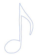
Quaver

Unsatisfied with the difficulty of drawing using a mouse, I used my Moleskine Notebook to draw the shape of a musical note (a quaver), exported it as “svg” (vector graphics) and wrote a small script to convert the svg to a parametric curve. Here is the shape I drew:

Here are the Fourier transforms with 6, 10, 20, 100, 400 and 1000 vectors: