Motivation

Let’s take a look at how we multiply two polynomials of degree \(N\): \[\begin{align*} f(x) &= 4x^{4}-2x^{3}-6x^{2}\ +4x\ +\ 3\\ g(x) &= -x^{4}+11x^{3}-9x^{2}+-1x\ +\ 6\\ \end{align*}\]

We can use the distributive property to multiply two polynomials and then sum up coefficients for identical terms. \[\begin{align*} f(x) &\cdot g(x) = \\ (4x^{4}-2x^{3}-6x^{2}\ +4x\ +\ 3) &\cdot (-x^{4}+11x^{3}-9x^{2}+-1x\ +\ 6) = \\ -4x^{8}+46x^{7}-52x^{6}-56x^{5} &+ 121x^{4}-9x^{3}-67x^{2}+21x+18 \end{align*}\]

However, this leads to \(O(N^2)\) operations to compute the coefficients. In this section, we are going to look at how we can accomplish polynomial multiplication in \(O(NlogN)\) using Fast Fourier Transform (FFT) (an algorithm to compute DFT). We will also look at how we can solve this problem in ~10 lines of code!

Polynomial Representations

A polynomial of degree \(n-1\) can be represented via:

• Coefficient Representation: \(n\) coefficients \([a_0, a_1, a_2, \cdots, a_{n-1}]\)
• Value Representation: \(n\) sample points \([(x_1, f(x_1)), (x_2, f(x_2)), \cdots, (x_{n-1}, f(x_{n-1}))]\)

Note that any \(n\) unique points uniquely identify one and only one polynomial of degree \(n-1\) (Interpolation Theorem).

Polynomial Multiplication

We observe that computing polynomial multiplication using the coefficients leads to \(O(N^2)\) operations. Now, let’s try the value representation.

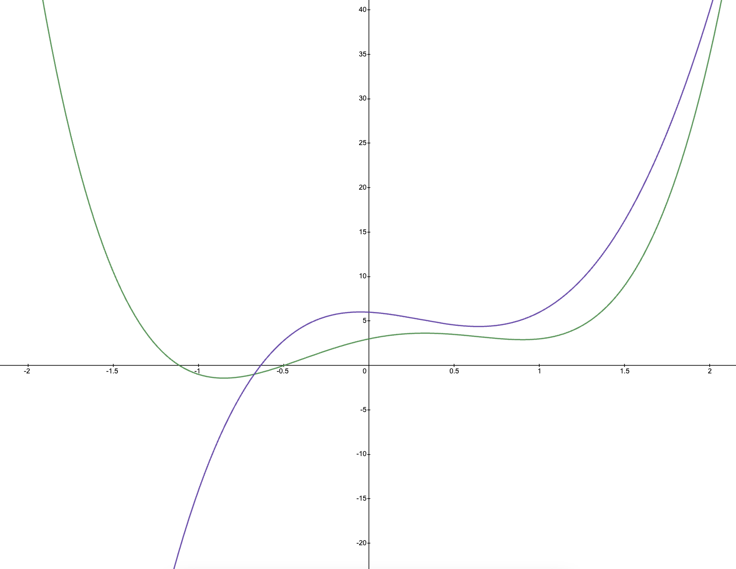
These are the polynomials f(x) and g(x) that we want to multiply:

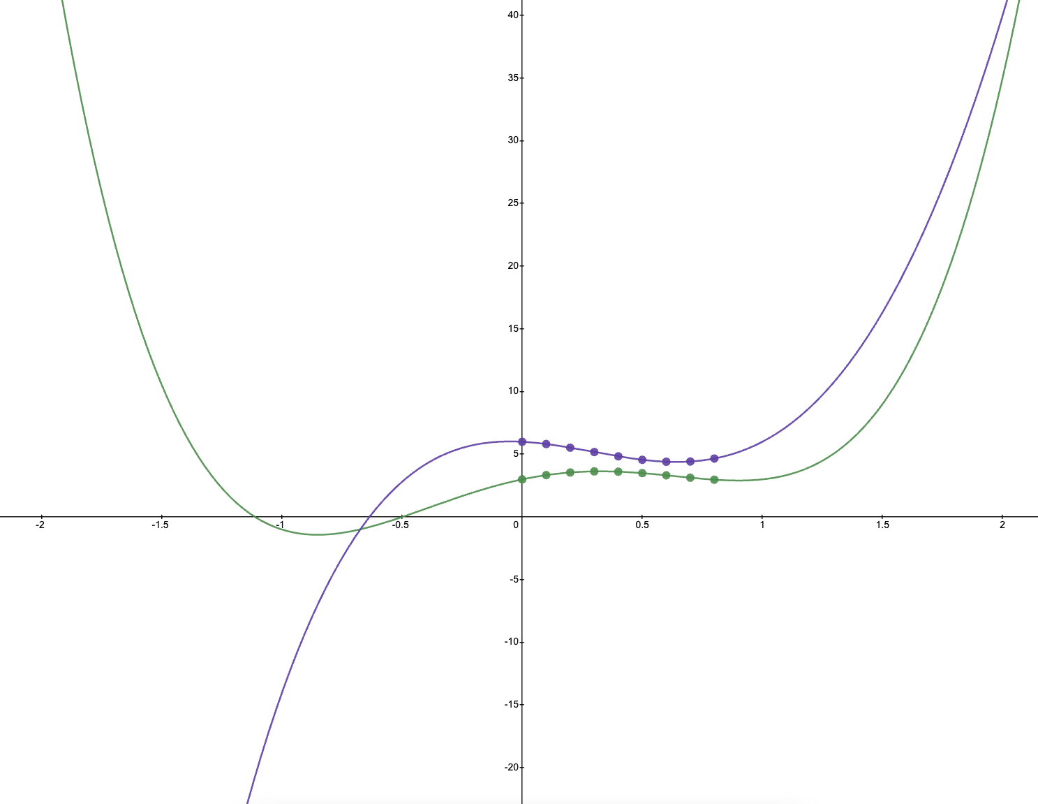
Step1: Sample \(n\) points on each polynomial (at the same x coordinates).

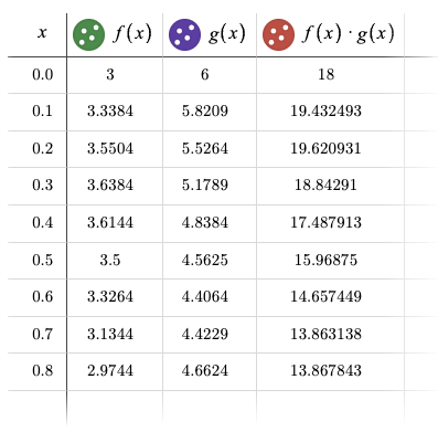
Step2: Compute the pairwise product of samples.

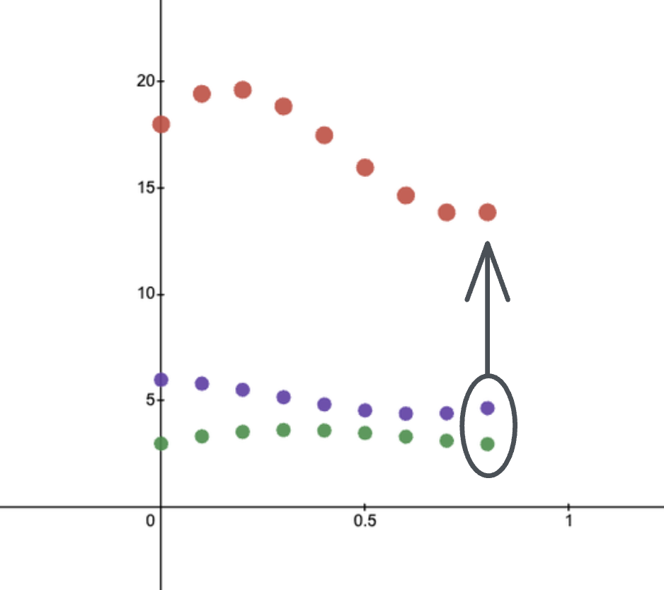
Step3: Find the unique polynomial of degree \(n-1\) (\(n\) coefficients) that goes through these \(n\) red points (interpolation).

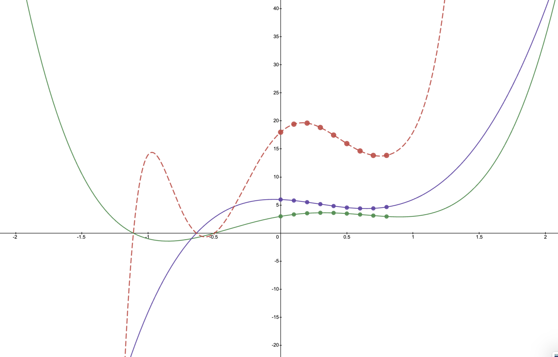
This new red curve is our polynomial \(f(x) \cdot g(x)\) and performing the multiplication using the value representation allowed us to multiply the two polynomials in \(O(N)\) operations.

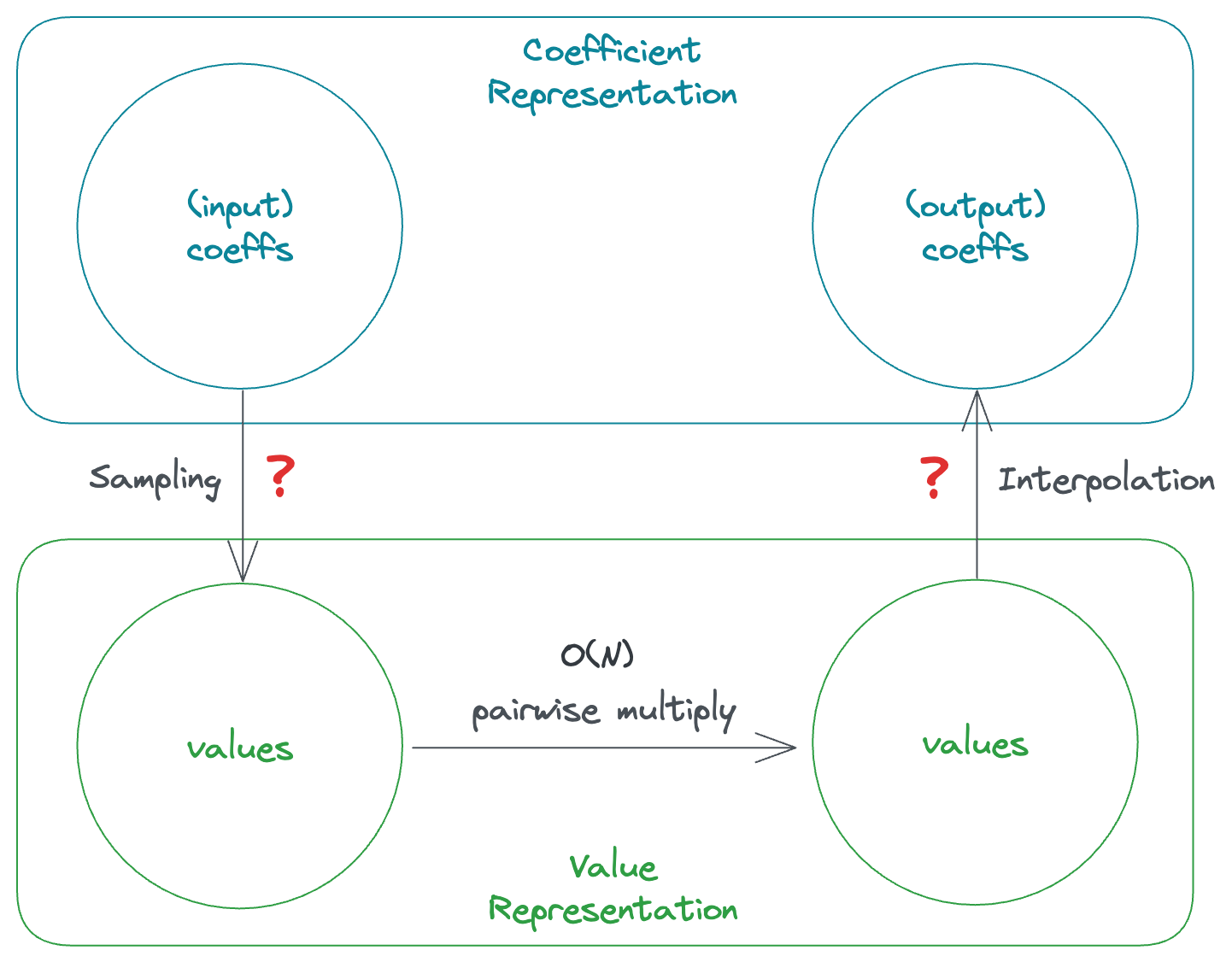
Now we need two magical operations to take us from the coefficient representation to the value representation and vice versa in less than \(O(N^2)\). This magical algorithm is called Fast Fourier Transform or FFT.

Fast Fourier Transform

Evaluation (DFT)

We know the result of multiplying two degree \(n\) polynomials is going to be of degree \(2n\), so we need to take \(2n+1\) samples. However, each sample (for example evaluating \(f(1)\)) requires \(O(n)\) operations and we need \(2n+1\) samples, resulting in an \(O(n^2)\) time complexity. On the other hand, we get to choose the set of \(x\)’s for which we want to sample \(f(x)\).

Observation

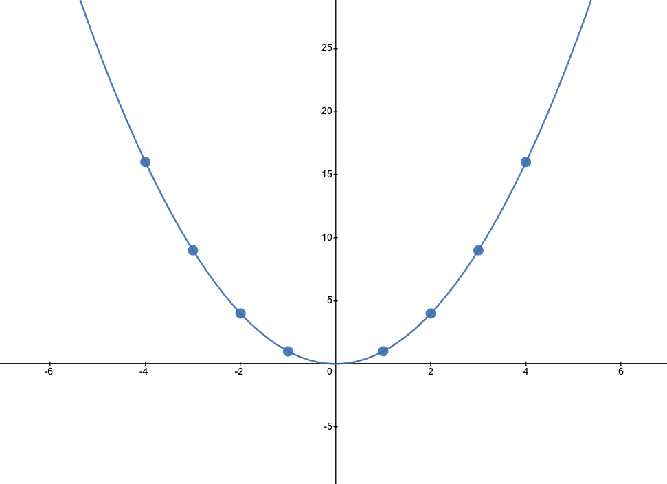
If we want to sample the function \(f(x) = x^2\), we can select specific samples by choosing positive values for x and their corresponding negative counterparts (given \(f(x)=f(-x)\)), thus saving half of the computation. Also, note that the same property holds for any even function.

Arbitrary Polynomials

Let’s say we want to evaluate the function \(f(x) = 4x^{4}-2x^{3}-6x^{2}+4x+3\), let’s start by isolating the terms with even and odd powers, and then factor out \(x\) from the odd powers (to make them all even) and call them \(F_e\) and \(F_o\) respectively: \[\begin{align*} F(x) &= \color{blue}{4x^{4}}\color{magenta}{-2x^{3}}\color{blue}{-6x^{2}}\color{magenta}{+4x}\color{blue}{+3}\\ F(x) &= \color{blue}{(4x^{4}-6x^{2}+3)} + \color{magenta}{(-2x^{3}+4x)}\\ F(x) &= \color{blue}{(4x^{4}-6x^{2}+3)} + \color{magenta}{x \cdot (-2x^{2}+4)}\\ F(x) &= \color{blue}{F_e(x^2)} + \color{magenta}{x F_o(x^2)} \end{align*}\]

Property 1: If we compute F(x) in this fashion, computing F(-x) becomes trivial. \[\boxed{ \begin{align*} F(x) &= F_e(x^2) + x F_o(x^2) \\ F(-x) &= F_e(x^2) - x F_o(x^2) \end{align*} }\]

Property 2: Note that \(F_e(x^2) = 4x^{4}-6x^{2}+3\) is actually a polynomial of degree 2! substituting \(x^2\) with \(v\) helps us see it better: \(F_e(v) = 4v^2-6v+3\).

Recap: We start with a function \(F(x)\) and pick our samples as positive and negative pairs. We only need to compute the positive samples, cutting down our problem from \(n\) to two smaller subproblems of size \(n/2\). Note that the sample size is reduced in half, as well as the degree of the polynomial. If we can make this work, we have an \(O(nlogn)\) recursive solution!

Challenge: The problem is as we go to recurse to the next step, when we decide to split our samples into positive and negative pairs \([\pm x'_1, \pm x'_2, ..., \pm x'_{n/4}]\), our new samples \([x_1^2, x_2^2, ..., x_{n/2}^2]\) cannot become negative, unless if we allow the samples to be complex numbers.

Complex Samples

We observed that if we pick a sample pair \(x_1=1\) and \(x=-1\), in the next step of recursion we need \(x^2 = 1\) and \(x^2 = -1\). In order to achieve \(x^2 = -1\), we also need to pick a sample pair of \(i\) and \(-i\). So, our four samples will be \([1, -1, i, -i]\). Note that these are the 4 solutions to the equation \(x^4=1\), which are called the 4th roots of unity.

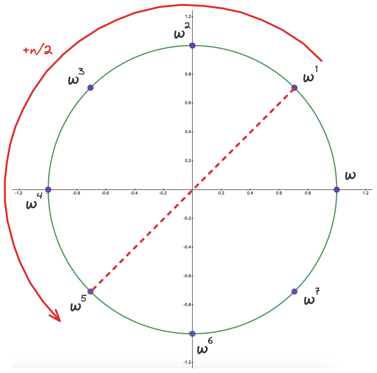
Nth Roots of Unity: In general, the solutions to the equation \(x^n=1\) are \([\omega^0, \omega^1, \cdots, \omega^{n-1}]\) where \(\boxed{\omega = e ^ {\frac{2 \pi i}{n}}}\). Below is the visualization of the roots for \(x^8=1\) on the complex plane.

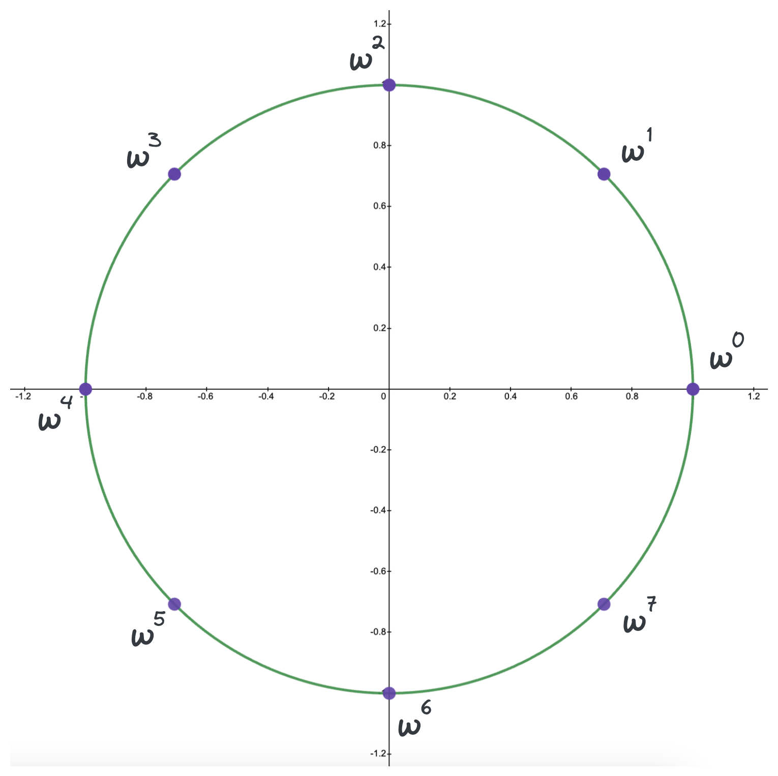
Basically, we are going to evaluate our polynomial at values \([\omega^0, \omega^1, \cdots, \omega^{n-1}]\) where the \(\pm\) pairs are \((w^i, w^{i+n/2})\) because \(-w^i = w^{i+n/2}\).

Implementation

We can implement this idea recursively in 10 lines of code. This implementation allows for evaluating \(n\) points from a degree \(n\) polynomial in \(O(nlog(n))\). Keep in mind that if you need more than \(n\) points sampled, just imagine you have a higher degree polynomial with the extra coefficients of \(0\).

import math, numpy as np

def FFT(c): # coefficients: [-1, 2, 3, 0] for 3x^2+2x-1
    n = len(c) # n must be a power of 2
    if n == 1:
        return c
    w = np.exp(2j * math.pi / n)
    fe, fo = FFT(c[::2]), FFT(c[1::2])
    f = [0] * n
    for i in range(n//2):
        f[i] = fe[i] + w**i * fo[i]
        f[i + n//2] = fe[i] - w**i * fo[i]
    return f

Interpolation

Having transformed the coefficients into points and performed pairwise multiplication, the next step involves determining the polynomial that passes through these points, a process known as “interpolation”. Although interpolation may initially appear to be a more challenging task, we will explore the close relationship between evaluation and interpolation, leading to a surprisingly simple solution.

DFT Matrix

Note that while sampling converts a polynomial (coefficients) to a set of points, interpolation acts as the inverse of that function converting points to the polynomial. Since sampling is a linear transformation, naturally the next step would be write the sampling/evaluation operation as a matrix and try to find its inverse to achieve the interpolation matrix.

Let’s take another look at sampling/evaluation for polynomial \(F(x) = c_0 + c_1x + c_2x^2 + \cdots + c_{n-1}x^{n-1}\) at points \([x_0, x_1, \cdots, x_{n-1}]\), using the Vandermonde matrix. \[\begin{pmatrix} \renewcommand\arraystretch{1.8} F(x_0)\\ F(x_1)\\ F(x_2)\\ \vdots\\ F(x_{n-1}) \end{pmatrix} = \begin{pmatrix} 1 & x_0 & x_0^2 & \dots & x_0^{n-1} \\ 1 & x_1 & x_1^2 & \dots & x_1^{n-1} \\ 1 & x_2 & x_2^2 & \dots & x_2^{n-1}\\ \vdots & \vdots & \vdots & \ddots & \vdots \\ 1 & x_{n-1} & x_{n-1}^2 & \dots & x_{n-1}^{n-1}\\ \end{pmatrix}\begin{pmatrix} c_0\\ c_1\\ c_2\\ \vdots\\ c_{n-1} \end{pmatrix}\]

And in the FFT algorithm, the i-th evaluation point is the corresponding root of unity (\(x_i = \omega^{i}\)), leading to the matrix below known as the Discrete Fourier Transform Matrix (The DFT Matrix). \[DFT = \begin{pmatrix} 1 & 1 & 1 & \dots & 1 \\ 1 & \omega & \omega^2 & \dots & \omega^{n-1} \\ 1 & \omega^2 & \omega^4 & \dots & \omega^{2(n-1)} \\ \vdots & \vdots & \vdots & \ddots & \vdots \\ 1 & \omega^{n-1} & \omega^{2(n-1)} & \dots & \omega^{(n-1)(n-1)} \end{pmatrix}\]

Inverse DFT Matrix

To be more precise, the DFT matrix also has a normalization factor of \(\frac{1}{\sqrt{n}}\) as shown below. \[\color{magenta}{\frac{1}{\sqrt{n}}} \, \begin{pmatrix} 1 & 1 & 1 & \dots & 1 \\ 1 & \omega & \omega^2 & \dots & \omega^{n-1} \\ 1 & \omega^2 & \omega^4 & \dots & \omega^{2(n-1)} \\ \vdots & \vdots & \vdots & \ddots & \vdots \\ 1 & \omega^{n-1} & \omega^{2(n-1)} & \dots & \omega^{(n-1)(n-1)} \end{pmatrix}\]

This normalization factor is often added to achieve a unitary matrix. Considering that the inverse of a unitary matrix is the conjugate transpose, and given our matrix is symmetric, we can achieve this by computing the conjugate of each term (negating the imaginary part). For the specific case of \(\omega = e ^ {\frac{2 \pi i}{n}}\) the conjugate would be \(e ^ {\frac{-2 \pi i}{n}}\) which is just \(\omega^{-1}\). So, the resulting matrix would be the same as the DFT matrix but with negative powers. \[\frac{1}{\sqrt{n}} \, \begin{pmatrix} 1 & 1 & 1 & \dots & 1 \\ 1 & \omega^{-1} & \omega^{-2} & \dots & \omega^{-(n-1)} \\ 1 & \omega^{-2} & \omega^{-4} & \dots & \omega^{-2(n-1)} \\ \vdots & \vdots & \vdots & \ddots & \vdots \\ 1 & \omega^{-(n-1)} & \omega^{-2(n-1)} & \dots & \omega^{-(n-1)(n-1)} \end{pmatrix}\]

Yet, it’s crucial to recognize that our initial DFT transformation was essentially an evaluation, devoid of the \(\frac{1}{\sqrt{n}}\) term. Therefore, to align with the problem at hand, we must provide another multiplier of \(\frac{1}{\sqrt{n}}\), resulting in the formulation: \[DFT^{-1} = \frac{1}{n} \, \begin{pmatrix} 1 & 1 & 1 & \dots & 1 \\ 1 & \omega^{-1} & \omega^{-2} & \dots & \omega^{-(n-1)} \\ 1 & \omega^{-2} & \omega^{-4} & \dots & \omega^{-2(n-1)} \\ \vdots & \vdots & \vdots & \ddots & \vdots \\ 1 & \omega^{-(n-1)} & \omega^{-2(n-1)} & \dots & \omega^{-(n-1)(n-1)} \end{pmatrix}\]

Multiplying this matrix by the evaluated points will yield the coefficients of the desired polynomial. \[\begin{pmatrix} c_0\\ c_1\\ c_2\\ \vdots\\ c_{n-1} \end{pmatrix} = \frac{1}{n} \, \begin{pmatrix} 1 & 1 & 1 & \dots & 1 \\ 1 & \omega^{-1} & \omega^{-2} & \dots & \omega^{-(n-1)} \\ 1 & \omega^{-2} & \omega^{-4} & \dots & \omega^{-2(n-1)} \\ \vdots & \vdots & \vdots & \ddots & \vdots \\ 1 & \omega^{-(n-1)} & \omega^{-2(n-1)} & \dots & \omega^{-(n-1)(n-1)} \end{pmatrix} \begin{pmatrix} \renewcommand\arraystretch{1.8} F(x_0)\\ F(x_1)\\ F(x_2)\\ \vdots\\ F(x_{n-1}) \end{pmatrix}\]

Now, comparing this with the original \(DFT\) matrix, the only differences are:

• negative powers
• multiply by \(\frac{1}{n}\) at the end

Full Implementation

With a one line change in the original implementation of our FFT function, we can have it compute inverse FFT as well. Just keep in mind that we have to divide the final result by \(n\) (which is why we introduced a separate function called IFFT).

import math, numpy as np

def FFT(c, inv=False):
    n = len(c) # coefficients: [-1, 2, 3, 0] for 3x^2+2x-1
    if n == 1: # n must be a power of 2
        return c
    w = np.exp(2j * math.pi / n * (-1 if inv else 1))
    fe, fo = FFT(c[::2], inv), FFT(c[1::2], inv)
    f = [0] * n
    for i in range(n//2):
        f[i] = fe[i] + w**i * fo[i]
        f[i + n//2] = fe[i] - w**i * fo[i]
    return f

def IFFT(c):
    f = FFT(c, inv=True)
    return [i / len(c) for i in f]

Testing

Let’s put our original polynomials to the test: \(\begin{align*} f(x) &= 4x^{4}-2x^{3}-6x^{2}\ +4x\ +\ 3\\ g(x) &= -x^{4}+11x^{3}-9x^{2}+-1x\ +\ 6\\ f(x) \cdot g(x) &= -4x^{8}+46x^{7}-52x^{6}-56x^{5} + 121x^{4}-9x^{3}-67x^{2}+21x+18 \end{align*}\)

Input

Note that the coefficients need to be sorted from the lowest power to the highest.

poly1 = [3, 4, -6, -2, 4]
poly2 = [6, -1, -9, 11, -1]

Code

Just keep in mind the output of IFFT is complex numbers, so we need to extract the real parts and round them to the nearest integer, since the types are float.

def make_power_of_two(arr):
    target_len = 2 ** (len(arr) - 1).bit_length()
    return arr + [0] * (target_len - len(arr))

def multiply_polynomials(poly1, poly2):
    # make them equal length and powers of 2
    target_len = 2 ** (len(poly1) + len(poly2) - 1).bit_length()
    poly1 += [0] * (target_len - len(poly1))
    poly2 += [0] * (target_len - len(poly2))

    p1, p2 = FFT(poly1), FFT(poly2)
    p_result = [p1[i] * p2[i] for i in range(target_len)]
    return IFFT(p_result)

Output

[18, 21, -67, -9, 121, -56, -52, 46, -4, 0, 0, 0, 0, 0, 0, 0]