Summary

In Building Ads Optimization we explored the process of building ads optimization and highlighted common pitfalls from an intuitive perspective. In this post, we’ll take a more theoretical approach, starting with the definition of an objective function and constraints, and then delving into solving the constrained optimization problem.

Optimization Formulation

Let’s work on finding an ads optimization solution that maximizes “total advertiser value” while adhering to the budget constraints of each ad.

Objective

Suppose every conversion \(i\) has an intrinsic value of \(V_i\) for the advertiser and the advertiser receives \(C_i\) conversions. The objective function we want to maximize would be the total advertiser value in the system as shown below: \[U = \sum_{i=1}^n V_i C_i\]

Unfortunately, we don’t know the true value of each conversion to the advertiser but let’s assume for now that this value (\(V_i\)) is somehow provided. Moreover, at the time of allocation, we cannot determine in advance whether displaying an ad to a user will result in a conversion (\(C_i\) remains unknown). However, by shifting our focus to the expected value of the utility function, we can work with the predicted likelihood of a conversion occurring instead. \[E(U) = E(\sum_{i=1}^n V_i C_i) = \sum_{i=1}^n V_i E(C_i)\] \[E(U) = \sum_{i=1}^n V_i \sum_{j=1}^{ops} p_{ij} x_{ij}\]

Where,

• \(p_{ij}\): \(p(conversion \mid impression)\) for ad \(i\) and ad opportunity \(j\)
• \(x_{ij}\): \(1\) if ad \(i\) is shown for the opportunity \(j\) otherwise \(0\)

Suppose we have an ML model that can predict \(p_{ij}\) for every \((ad, opportunity)\) and these predictions are accurate (the model is calibrated).

Constraints

Let’s suppose we charge every advertiser exactly the amount of value they receive (\(V_i\)) upon each conversion. Alternatively we can charge them the expected value upon each ad impression \(j\): \[price_j = V_i p_{ij} x_{ij}\]

Now, the spend of each ad \(i\) can be written as: \[spend_i = \sum_j^{ops} V_i p_{ij} x_{ij}\]

Finally, we have our \(n\) constraints to ensure no ad exceeds their budget: \[\forall i \sum_j^{ops} V_i p_{ij} x_{ij} \leq B_i\]

Note: this pricing strategy has incentive compatibility issues that we will address later on.

The Optimization Formulation

Now, let’s consolidate everything and in line with common practices in the optimization domain, we express the objective as a minimization problem and the constraint as an inequality with respect to zero. \[\begin{equation} \begin{aligned} \text{Minimize} \quad & -\sum_{i=1}^n V_i \sum_{j=1}^{ops} p_{ij} x_{ij} \\ \text{subject to} \quad & \forall i \sum_j^{ops} V_i p_{ij} x_{ij} - B_i \leq 0 \end{aligned} \end{equation}\]

Solution

In our optimization formulation, note that \(x_{ij}\) represents the ad/opportunity allocation where \(1\) means we show ad \(i\) in opportunity \(j\) and \(0\) means we don’t show the ad. Now, let’s see how we can find the optimal values for \(x_ij\) to not violate any of the constraints while minimizing the objective function.

The Lagrange Method

A widely used approach to solving constrained optimization problems is the Lagrange method, which identifies points where the gradient of the constraint is parallel to the gradient of the objective function. Take a look at this video Utility Maximization with Lagrange Method to better understand how it works on a simple example.

The Lagrange function is defined by incorporating all constraints into the objective function and assigning a multiplier \(\lambda_j\) to each constraint \(j\). \[\mathcal{L}(x, \lambda) = -\sum_{i=1}^n V_i \sum_{j=1}^{ops} p_{ij} x_{ij} + \sum_i^n \lambda_i \sum_j^{ops} V_i p_ {ij} x_{ij} - B_i\]

Next, we need to compute the partial derivatives with respect to each unknown variable (\(x_{ij}\) and \(\lambda_i\)) and set them to zero and then solve the resulting system of equations. \[\begin{equation} \begin{aligned} \forall x_{ij} & : \frac{\partial\mathcal{L}(x, \lambda)}{\partial x_{ij}} = 0 \\ \forall \lambda_{i} & : \frac{\partial\mathcal{L}(x, \lambda)}{\partial \lambda_{i}} = 0 \end{aligned} \end{equation}\]

However, this results in a large system of equations that is computationally infeasible and impractical, especially considering the dynamic nature of the problem we are trying to solve.

Lagrangian Relaxation

Lagrangian relaxation is a technique used in optimization to find approximate solutions to complex problems. The core idea behind Lagrangian relaxation involves relaxing the constraints of an optimization problem by incorporating them into the objective function using Lagrange multipliers, allowing them to be violated but associating a cost to those violations (via the lambda multipliers).

In Lagrangian relaxation, we relax the constraints \(g_i(x) \leq 0\) by incorporating them into the objective function using Lagrange multipliers \(\lambda_i \geq 0\). So, the Lagrangian function is defined as: \[\mathcal{L}(x, \lambda) = f(x) + \sum_{i=1}^{m} \lambda_i g_i(x)\]

Let’s see what happens if we try to maximize the Lagrange function: \[\max_{\lambda_i \geq 1} \mathcal{L(x, \lambda)} = \left\{ \begin{array}{ll} f(x) & \text{if } \, \, \forall i \, g_i(x) \leq 0, \\ \infty & \text{if } \, \, otherwise. \end{array} \right.\]

Now, observe that we can eliminate the infinity case by minimizing the expression above, leading to a formulation equivalent to our primal formulation. \[p^* = \min_{x} \max_{\lambda_i \geq 0} \mathcal{L}(x, \lambda)\]

The Dual of Lagrange

We have derived an equivalent formulation of our optimization problem without constraints, where the solution would match that of the original problem. Now to significantly simplify and solve this problem, we transform it into its dual form, also known as the Lagrangian Dual Problem. This is done by simply interchanging the “min” and “max” operations.

Primal form: \[\color{black}{p^* =} \,\, \color{blue}{\min_{x}} \,\, \color{green}{\max_{\lambda_i \geq 0}} \,\, \color{black}{\mathcal{L}(x, \lambda)}\]

Dual form: \[\color{black}{d^* =} \,\, \color{green}{\max_{\lambda_i \geq 0}} \,\, \color{blue}{\min_{x}} \,\, \color{black}{\mathcal {L}(x, \lambda)}\]

It can be easily shown that \(p^* \geq d^*\) (known as the weak duality) for any optimization problem. Solving the dual problem provides a lower bound on the primal and the difference between them is known as the duality gap. To prove strong duality, we would need to demonstrate that the duality gap is zero; however, we will skip that step for now.

The real power of the Dual of Lagrange is (from Convex Optimization by Boyd):

Since the dual function is the pointwise infimum of a family of affine functions of (λ, ν), it is concave, even when the problem (5.1) is not convex.

Since the dual function is the pointwise infimum of a family of affine functions of (λ, ν), it is concave, even when the problem (5.1) is not convex.

This is very important because the dual form of the Lagrange problem is always concave, ensuring a unique global optimum, which allows for the use of gradient ascent to solve it, regardless of the original problem’s properties (more details).

Auction and Pacing

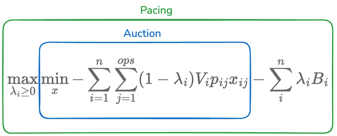
It’s now time to solve the dual of the Lagrange: \[\begin{equation} \begin{aligned} & \max_{\lambda_i \geq 0} \min_{x} \mathcal{L}(x, \lambda) \\ & = \max_{\lambda_i \geq 0} \min_{x} -\sum_{i=1}^n V_i \sum_{j=1}^{ops} p_{ij} x_{ij} + \sum_i^n \lambda_i \left( \sum_j^{ops} V_i p_{ij} x_{ij} - B_i \right) \\ & = \max_{\lambda_i \geq 0} \min_{x} -\sum_{i=1}^n \sum_{j=1}^{ops} V_i p_{ij} x_{ij} + \sum_i^n \sum_j^{ops} \lambda_i V_i p_{ij} x_{ij} - \sum_i^{n} \lambda_i B_i \\ & = \max_{\lambda_i \geq 0} \min_{x} -\sum_{i=1}^n \sum_{j=1}^{ops} (1 - \lambda_i) V_i p_{ij} x_{ij} - \sum_i^{n} \lambda_i B_i \\ \end{aligned} \end{equation}\]

Auction

Let’s first solve the inner minimization, assuming fixed values of \(\lambda_i\) (from the outer maximization). Note that \(\sum_i^{n} \lambda_i B_i\) will be constant and we mainly have to solve for: \[\min_{x} - \sum_{i=1}^n \sum_{j=1}^{ops} (1 - \lambda_i) V_i p_{ij} x_{ij}\]

Alternatively, \[\max_{x} \sum_{i=1}^n \sum_{j=1}^{ops} (1 - \lambda_i) V_i p_{ij} x_{ij}\]

This maximization needs to be solved with a valid set of \(x_{ij}\) values, meaning for every request only one ad can have this value set to \(1\) and the rest would be \(0\). The solution would simply be achieved by picking the ad with the highest value of \((1 - \lambda_i) V_i p_{ij}\).

Note that this is analogous to running an “Auction” where each ad participates with the bid of: \[bid = \lambda_i' V_i p_{ij}\]

Where:

• \(\lambda_i' = (1 - \lambda_i)\) is the pacing (bid shading) multiplier which should be between \(0\) and \(1\).
• \(V_i\) is the intrinsic value of a conversion to the advertiser
• \(p_{ij}\) is the probability of conversion happening if we show the ad to this user

Note: The auction we designed here is not incentive compatible as it encourages advertisers to lower their \(V_i\) input in the system to achieve better ROI. In order to make the auction incentive compatible, we need to address pricing differently but we won’t cover that in this post. The beauty of having an incentive compatible system is that advertiser’s incentive (higher ROI) becomes aligned with our incentive (knowing the true value \(V_i\)) and it helps with our assumption on \(V_i\) representing the intrinsic value of each conversion to the advertiser, prevents manipulations from advertisers to achieve better results and overall creates a healthy ads ecosystem.

Pacing

Since we already know how to maximize the inner optimization, let’s denote the optimal allocation for the inner loop as \(x^*\) . Now, let’s focus on how we can determine the optimal values of \(\lambda_i\) to: \[\max_{\lambda_i \geq 0} \mathcal{L}(x^*, \lambda)\]

As we discussed earlier, a key advantage of the Lagrange dual problem is that the dual function is always concave, regardless of the original objective or constraints. This allows us to solve it efficiently using Gradient Ascent by repeating these steps:

1. start with initial values of \({\lambda_0, \lambda_1, ..., \lambda_n}\)
2. Compute the partial derivative with respect to each \(\lambda_i\)
3. Update values of \(\lambda_i\) towards the gradient using: \(\lambda_{i} = \lambda_{i} - \eta \left(\frac{\partial \mathcal{L}(x^*, \lambda)}{\partial \lambda_i} \right)\)

To better understand step (3), let’s compute the partial derivative of the Lagrange function (note that terms without \(\lambda_i\) in them will become zero): \[\begin{equation} \begin{aligned} & \frac{\partial \mathcal{L}(x^*, \lambda)}{\partial \lambda_i} \\ & = \frac{\partial \left[-\sum_{i=1}^n \sum_{j=1}^{ops}(1 - \lambda_i) V_i p_{ij} x_{ij} - \sum_i^{n} \lambda_i B_i \right] }{\partial \lambda_i}\\ & = \sum_{j=1}^{ops} V_i p_{ij} x_{ij} \\ & = S_i - B_i \end{aligned} \end{equation}\]

Putting everything together the step (3) becomes: \[\lambda_{i} = \lambda_{i} + \eta \, (B_i - S_i)\]

Where,

• \(S_i\) is the spend of ad \(i\)
• \(B_i\) is the budget of ad \(i\)

Simulation

Putting this all together to solve for the optimal allocation, we can assume a simple solution consisting of only two ads with different budgets and figure out the optimal allocation. Let’s use this data structure to store data regarding an ad:

class Ad:
    def __init__(self, max_bid, budget, p):
        self.max_bid = max_bid
        self.budget = budget
        self.p = p
        self.spend = 0
        self.lam = 0.5

    def calc_bid(self, idx):
        return self.lam * self.max_bid * self.p[idx]

    def deliver(self, price):
        self.spend += price

    def update_pacing(self):
        self.lam = self.lam + 0.0001 * (self.budget - self.spend)
        self.lam = max(0, min(1, self.lam))

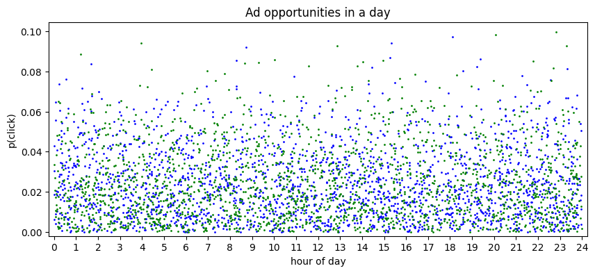
Then we create two instances of ads with the same max_bid (\(V_i\)) but the second one with a much smaller budget, and run the simulation of auction and pacing (gradient ascent), 500 times.

ads = [Ad(max_bid=10, budget=100, p=y1), 
       Ad(max_bid=10, budget=5, p=y2)]

floor = 100/1000
for i in range(500):
    for j in range(N):
        # auction
        result = sorted(ads, key=lambda x: x.calc_bid(j))
        winner = result[-1]
        price = winner.calc_bid(j)
        if price >= floor:
            winner.deliver(price)
    
    # pacing
    for ad in ads:
        ad.update_pacing()
        ad.spend = 0

Note that each ad values an opportunity differently (a value derived from an ML model), so values for ad1 is shown in blue and for ad2 in green.

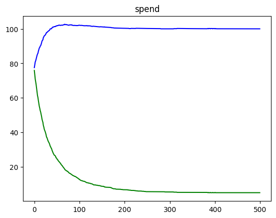
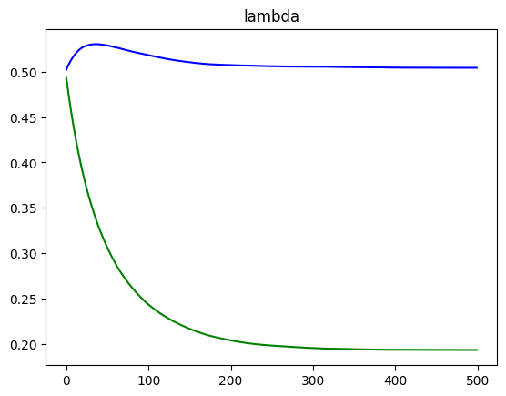
We can see how running the simulation results in spend converging to the budget of each ad, as well as lambda converging to the optimal value for each ad.

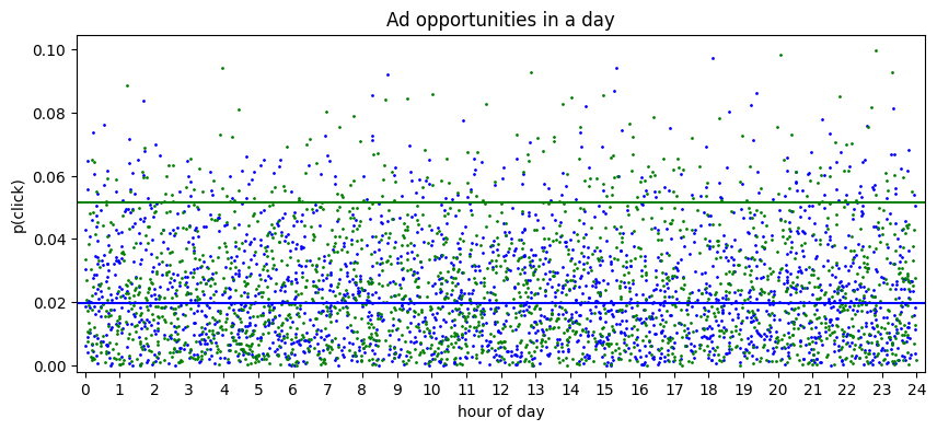
Now, in order to show the actual selection of opportunities, note that each ad in isolation would win if \(\lambda_i V_i p_{ij} >= floor\) or alternatively if: \[p_{ij} >= \frac{floor}{\lambda_i V_i}\]

So we visualize \(\frac{floor}{\lambda_i V_i}\) as a horizontal line. Note how the line with a lower budget becomes more selective towards which opportunities it considers (via a higher horizontal line).

Conclusion

In this post, we explored how to determine the optimal allocation of \(M\) ad opportunities across \(N\) ads, each with different budgets and max bids. In practice, additional constraints like targeting and frequency capping come into play as well. We delved into the theory behind this constrained optimization problem, which results in a max/min optimization. The inner optimization corresponds to the auction, while the outer optimization becomes pacing. The outer optimization is guaranteed to be concave, allowing for a straightforward solution using gradient ascent.

While the auction simply picks the highest bidding ad in the auction, the pacing algorithm in reality is more involved as we don’t have access to the opportunities in the future, so we need to predict them by predicting the future based on the historical data points. So, a real pacing algorithm in production basically is constantly trying to solve this hill climbing algorithm based on its knowledge so far and the prediction of the future, while adapting to advertiser changes (ex: budget changes).

A pacing algorithm can be effectively implemented by calculating the desired spend profile, and then adjusting the pacing multipliers to achieve the target spend. In a real production system, there is a lot of uncertainty and moving parts including the target itself. So the common approach involves leveraging a closed-loop control system to continuously refine the pacing multiplier to reach the desired spend.

Interesting takeaways:

• It looks like we are picking the highest bidder ad in the auction, but we’re not really picking the best ad for the user. Pacing is really setting the baseline for the bid, choosing which opportunities to select for this ad.
• The goal of budget pacing is way more than spending the budget smoothly. Notice that while probabilistic pacing would result in a smooth spend curve, it provides little to no benefits when it comes to ads performance.