Motivation
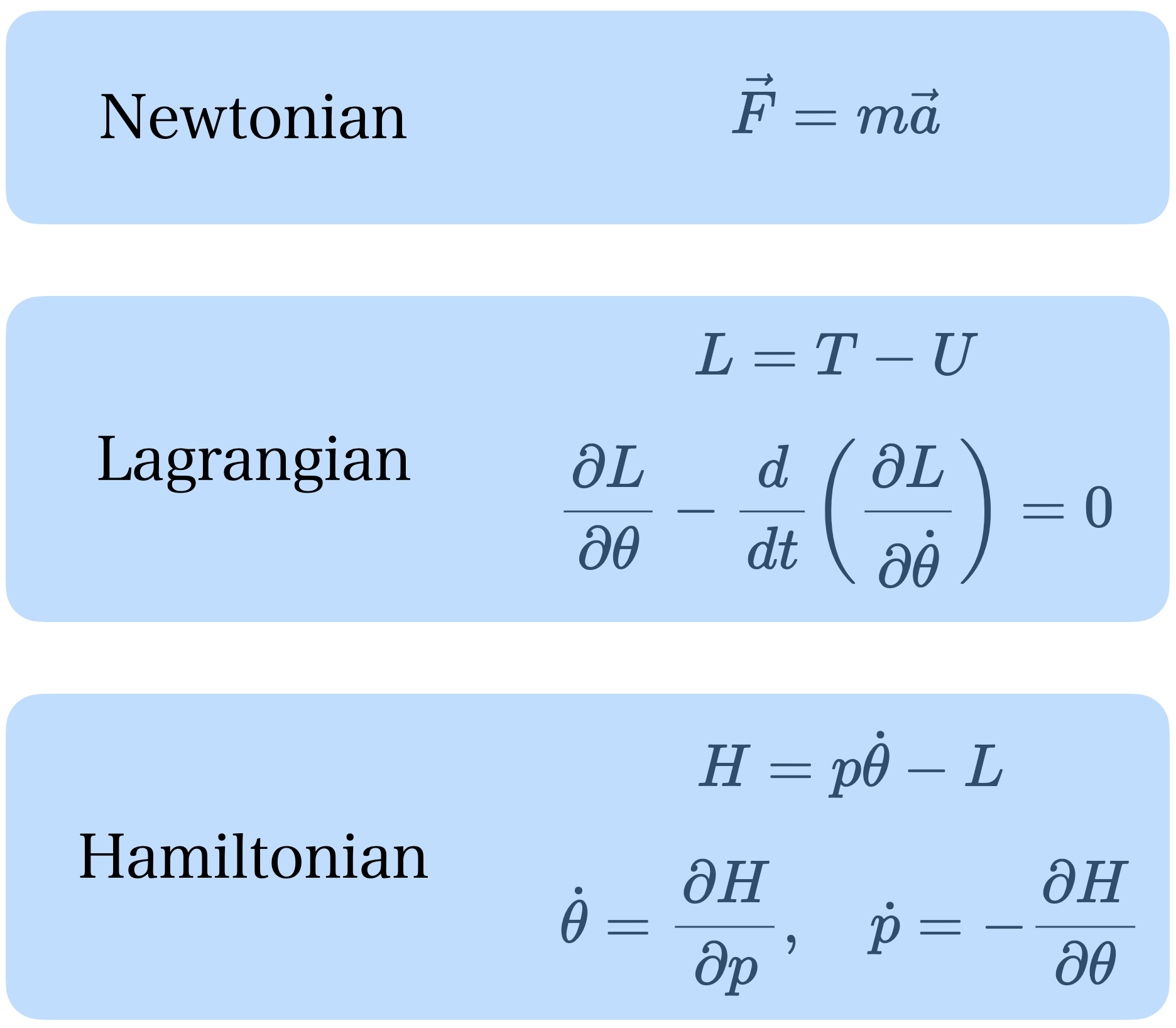
Let’s explore how we can simulate physical phenomena in Python by building everything from scratch, step by step. When it comes to modeling physical systems, there are three primary approaches: the Newtonian, the Lagrangian, and the Hamiltonian.
- The Newtonian approach, grounded in \(F = ma\) , focuses on forces and accelerations to describe motion.
- The Lagrangian approach, based on the principle of least action, emphasizes energy and leads us to the elegant Euler-Lagrange equation.
- The Hamiltonian approach reformulates the problem further using generalized coordinates and momenta, offering powerful insights in modern physics.
While Newton’s laws are intuitive, the Lagrangian method is more elegant, versatile and easier to use for simulation purposes. Derived from the principle of least action, introduced by Pierre-Louis Maupertuis in 1744 and later refined by Leonhard Euler and Joseph-Louis Lagrange, it provides a universal framework that simplifies simulations by focusing on energy rather than forces.
Using the Euler-Lagrange equation, we can mathematically model and simulate physical systems, from a pendulum’s swing to the orbits of planets. If you’re curious about the elegance of the principle of least action, check out this incredible video by Veritasium. Inspired by this, we’re going to explore how to bring these ideas to life with Python!
Ordinary Differential Equations (ODEs)
ODEs are key to physical simulations as they model changes in motion step-by-step, reflecting how forces like gravity, tension or friction shape systems over time. This relative approach simplifies modeling complex interactions, allowing precise simulations through numerical solutions.
Lagrangian Mechanics
The solution to a Lagrangian typically provides the equations of motion for a system. In analytical mechanics, you start with the Lagrangian function \(\mathcal{L} = T - U\) (where T is the kinetic energy and U is the potential energy) and then use the Euler–Lagrange equations: \[\frac{d}{dt} \left(\frac{\partial \mathcal{L}}{\partial \dot{q}_i}\right) - \frac{\partial \mathcal{L}}{\partial q_i} = 0\]
to derive the dynamics. These equations tell you how the generalized coordinates \(q_i\) evolve over time. In other words, solving the Lagrangian gives you the trajectory or time evolution of the system’s configuration.
To summarize, we follow these three steps:
- Identify a minimal set of independent variables (generalized coordinates) that uniquely describe the configuration of our system. These coordinates can be angles, distances, etc. (these are \(q_i\) in the above statement)
- Construct the Lagrangian as \(\mathcal{L} = T - U\) where:
- \(T\): the kinetic energy of the system
- \(U\): the potential energy of the system
- Obtain the ODE via the Euler-Lagrange equation: \(\frac{\partial \mathcal{L}}{\partial \theta} - \frac{d}{dt} \left( \frac{\partial \mathcal{L}}{\partial \dot{\theta}} \right) = 0\)
Simple Pendulum
Let’s look into how we can simulate a simple pendulum using the Lagrangian mechanics and visualize it in Python.
Lagrangian Steps
Step 1: Generalized Coordinates
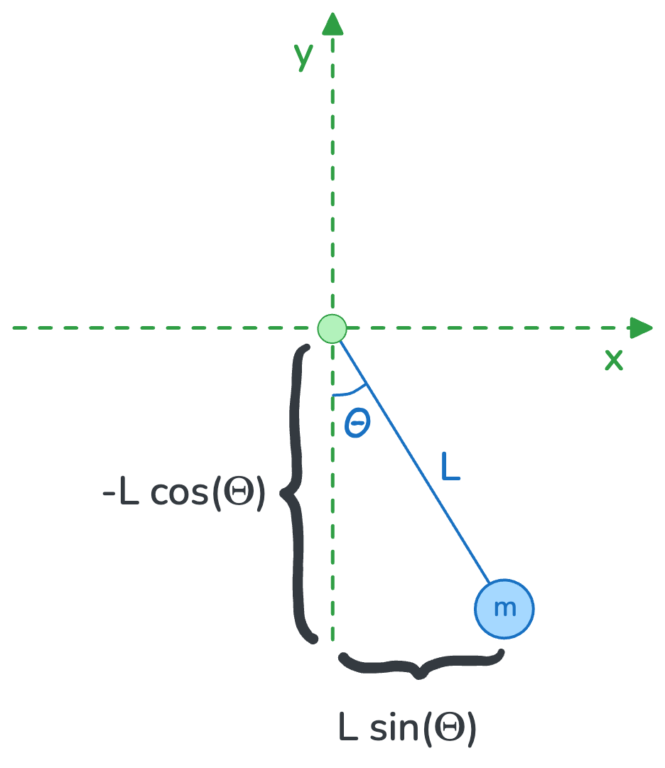
We can use the polar coordinate system and represent the state of the pendulum at any point in time with:
- \(\theta\): The angle from the y-axis line
- \(m\): The mass of the object hanging from the pendulum
- \(L\): The length of the pendulum, which is constant in our simulation
We can write the cartesian coordinates of the pendulum object as: \[\begin{equation} \begin{aligned} x_m &= L \sin \theta \\ y_m &= -L \cos \theta \end{aligned} \end{equation}\]
And the first derivatives w.r.t time (notice \(\theta\) is a function of time, so we need to apply the chain rule): \[\begin{equation} \begin{aligned} \dot{x}_m &= L \dot{\theta} \cos \theta \\ \dot{y}_m &= L \dot{\theta} \sin \theta \\ \end{aligned} \end{equation}\]
Step 2: Construct the Lagrangian
We can write down the kinetic and potential energy in the system and subtract them to find the Lagrangian.
- Kinetic Energy:
- Potential Energy:
- The Lagrangian:
Step 3: The Euler-Lagrange ODE
Now that we have \(\mathcal{L}\), let’s solve the Euler-Lagrange differential equation: \[\begin{equation} \begin{aligned} &\frac{d}{dt} \left( \frac{\partial \mathcal{L}}{\partial \dot{\theta}} \right) - \frac{\partial \mathcal{L}}{\partial \theta} = 0 \\ &\frac{d}{dt} \left( \frac{\partial }{\partial \dot{\theta}} \left[ mL(\frac{1}{2}L\dot\theta^2 + g\cos(\theta)) \right] \right) - \frac{\partial }{\partial \theta} \left[ mL(\frac{1}{2}L\dot\theta^2 + g\cos(\theta)) \right] = 0 \\ &\frac{d}{dt} \left( \frac{\partial }{\partial \dot{\theta}} \left[ \cancel{mL}(\frac{1}{2}L\dot\theta^2 + g\cos(\theta)) \right] \right) - \frac{\partial }{\partial \theta} \left[ \cancel{mL}(\frac{1}{2}L\dot\theta^2 + g\cos(\theta)) \right] = 0 \\ &\frac{d}{dt} \left( \frac{\partial }{\partial \dot{\theta}} \left[\frac{1}{2}L\dot\theta^2 + g\cos(\theta) \right] \right) - \frac{\partial }{\partial \theta} \left[ \frac{1}{2}L\dot\theta^2 + g\cos(\theta) \right] = 0 \\ &\frac{d}{dt} \left( \frac{\partial }{\partial \dot{\theta}} \left[\frac{1}{2}L\dot\theta^2\right] + \frac{\partial }{\partial \dot{\theta}} \Bigl[ g\cos(\theta) \Bigr] \right) - \left[\frac{\partial }{\partial \theta} \left[ \frac{1}{2}L\dot\theta^2 \right] + \frac{\partial }{\partial {\theta}} \Bigl[ g\cos(\theta) \Bigr] \right] = 0 \\ &\frac{d}{dt} \left( L\dot\theta + 0 \right) - \Bigl[0 + (-g\sin(\theta)) \Bigr] = 0 \\ &\frac{d}{dt} \left( L\dot\theta \right) + g\sin(\theta) = 0 \\ &L\ddot\theta + g\sin(\theta) = 0 \\ \end{aligned} \end{equation}\] \[\boxed{\ddot\theta = -\frac{g\sin\theta}{L}}\]
Simulation
Now that we have the equation of motion for the single pendulum, let’s look at how we can simulate and visualize it using Python.
Bare-Metal Simulation
Given a time step \(dt\) , we can numerically compute the state of the pendulum at discrete time intervals. We begin by initializing the angle \(\theta\) and angular velocity \(\dot{\theta}\) with their respective initial values. Then, we iteratively update their values, as shown below:dt = 1 / 20
theta_dot = init_theta_dot
theta = init_theta
while True:
theta_dot_dot = - g * math.sin(theta) / L
theta_dot += theta_dot_dot * dt
theta += theta_dot * dt
The full simulation code would look like:import math
import matplotlib.pyplot as plt
from matplotlib.animation import FuncAnimation, FFMpegWriter
from IPython.display import HTML
plt.style.use('default')
def get_xy_pos(theta, L):
return (L * math.sin(theta), -L * math.cos(theta))
# pendulum parameters
g = 9.8
L = 1
init_theta = math.pi / 5
init_theta_dot = 0
# time step
dt = 1 / 20
# initial conditions
theta_dot = init_theta_dot
theta = init_theta
# figure setup
fig, ax = plt.subplots()
ax.set_xlim(-L - 0.1, L + 0.1)
ax.set_ylim(-L - 0.3, + 0.1)
ax.set_aspect('equal')
ax.set_xticks([])
ax.set_yticks([])
# pendulum visuals
line, = ax.plot([], [], 'o-', color='gray')
ball, = ax.plot([], [], 'o', color='green', markersize=20)
# update function for animation
def animate(frame):
global theta, theta_dot
# update angular acceleration, velocity, and position
theta_dot_dot = - g * math.sin(theta) / L
theta_dot += theta_dot_dot * dt
theta += theta_dot * dt
# update pendulum position
x, y = get_xy_pos(theta, L)
line.set_data([0, x], [0, y])
ball.set_data([x], [y])
return line,
# Create the animation
ani = FuncAnimation(fig, animate, frames=430, interval=dt*800, blit=True)
ani.save('pendulum.gif', writer=FFMpegWriter(fps=30))
HTML(ani.to_html5_video())
Result:
Simulation using Scipy
Given the results of the ODE that we calculated as \(\ddot\theta = -\frac{g\sin\theta}{L}\), we can let the python library scipy help us with the numerical simulation. In particular, we will leverage the library scipy.integrate.solve_ivp.import math
import numpy as np
from scipy.integrate import solve_ivp
import matplotlib.pyplot as plt
from matplotlib.animation import FuncAnimation
from IPython.display import HTML
def get_pend_pos(theta, L):
return (L * math.sin(theta), -L * math.cos(theta))
# pendulum parameters
g = 9.8
L = 1
init_theta = math.pi / 5
init_theta_dot = 0
# f: [theta, theta_d]
def pendulum_ODE(t, f):
return (f[1], -g * math.sin(f[0])/L)
sol = solve_ivp(
fun=pendulum_ODE,
t_span=[0, 3],
y0=(init_theta, init_theta_dot),
t_eval=np.linspace(0, 3, 120*5)
)
theta_arr, theta_dot_arr, t_arr = sol.y[0], sol.y[1], sol.t
# figure setup
fig, ax = plt.subplots()
ax.set_xlim(-L - 0.1, L + 0.1)
ax.set_ylim(-L - 0.3, + 0.1)
ax.set_aspect('equal')
ax.set_xticks([])
ax.set_yticks([])
# pendulum visuals
line, = ax.plot([], [], 'o-', color='gray')
ball, = ax.plot([], [], 'o', color='green', markersize=20)
# Update function for animation
def animate(i):
x, y = get_pend_pos(theta_arr[i], L)
line.set_data([0, x], [0, y])
ball.set_data([x], [y])
return line,
# Create the animation
ani = FuncAnimation(fig, animate, frames=len(t_arr), interval=5, blit=True)
# Display the animation as an HTML5 video
HTML(ani.to_html5_video())
Solving the ODE
As you have noticed, the step 3 of the lagrangian was not very easy. So, let’s leverage the symbolic math library sympy for that:from sympy import *
from sympy.physics.mechanics import *
init_vprinting()
m, g, l, t = symbols('m g L t')
theta = dynamicsymbols('theta')
x,y = l*sin(theta), -l*cos(theta)
x_d, y_d = diff(x, t), diff(y, t)
theta_d = diff(theta, t)
theta_dd = diff(theta_d, t)
# Lagrangian
T = 1/2 * m * (x_d ** 2 + y_d ** 2)
U = m * g * y
L = T - U
eqn = diff(diff(L, theta_d), t) - diff(L, theta)
sln = solve(eqn, theta_dd)
Eq(theta_dd, sln[0])
Or to see it in a format understandable by scipy:mat_d = Matrix([theta_d, theta_dd])
Eq(mat_d, Matrix([theta_d, sln[0]]))
Spring Pendulum
Now, let’s use everything we have learned so far to simulate a spring pendulum!
Lagrangian Steps
Step 1: Generalized Coordinates
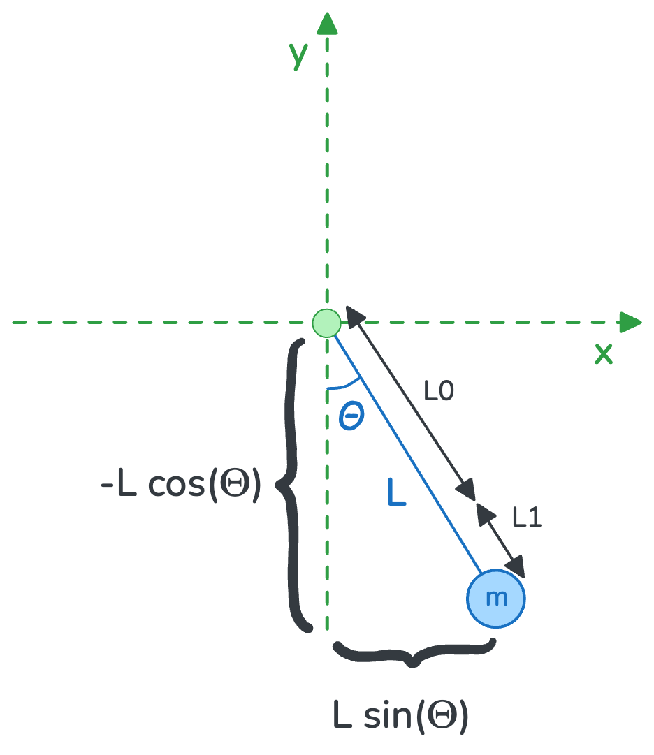
Suppose the spring has a natural length of L0 (with no weight attached) and at any point in time, it can be expanded by L1 due to forces. The total length of the pendulum at any point in time would be: L = L0 + L1
We can write the cartesian coordinates of the pendulum object as: \[\begin{equation} \begin{aligned} x_m &= (L_0 + L_1) \sin \theta \\ y_m &= -(L_0 + L_1) \cos \theta \end{aligned} \end{equation}\]
Note that both \(\theta\) and \(L1\) are a function of time. So, the derivatives with respect to time would be: \[\begin{equation} \begin{aligned} \dot{x}_m &= \dot{L_1} \sin \theta + (L_0 + L_1) \dot{\theta} \cos \theta \\ \dot{y}_m &= -\dot{L_1} \cos \theta + (L_0 + L_1) \dot{\theta} \sin \theta \\ \end{aligned} \end{equation}\]
Step 2: Construct the Lagrangian
We can write down the kinetic and potential energy in the system and subtract them to find the Lagrangian.
- Kinetic Energy:
- Potential Energy:
- The Lagrangian:
Step 3: The Euler-Lagrange ODE
Let’s use sympy:from sympy import symbols, Function, diff, sin, cos, solve, Eq, init_printing
from sympy.physics.mechanics import dynamicsymbols
init_vprinting()
# Define symbols
m, g, k, L0 = symbols('m g k L0') # constants
theta, L1 = dynamicsymbols('theta L1') # functions of time
theta_d = diff(theta, 't') # first derivative
theta_dd = diff(theta_d, 't') # second derivative
L = L0 + L1
L1_d = diff(L1, 't')
L1_dd = diff(L1_d, 't')
# Define coordinates
x = L * sin(theta)
y = -L * cos(theta)
# Velocities
x_d = diff(x, 't')
y_d = diff(y, 't')
# Kinetic energy
T = 1/2 * m * (L1_d**2 + (L)**2* theta_d**2)
# Potential energy
V = 1/2 * k * L1**2 - m * g * L * cos(theta)
# Lagrangian
Lagrangian = T - V
# Euler-Lagrange equations of motion
eqn_theta = diff(diff(Lagrangian, theta_d), 't') - diff(Lagrangian, theta)
eqn_L1 = diff(diff(Lagrangian, L1_d), 't') - diff(Lagrangian, L1)
# Solve both
sln = solve([eqn_theta, eqn_L1], [theta_dd, L1_dd])
# Show the solution
f = Matrix([theta_d, sln[theta_dd], L1_d, sln[L1_dd]])
f = simplify(f)
mat = Matrix([theta, theta_d, L1, L1_d])
mat_d = diff(mat, t)
Eq(mat_d, f)
Simulation
import math
import numpy as np
from sympy import *
from sympy.physics.mechanics import *
from scipy.integrate import solve_ivp
import matplotlib.pyplot as plt
from matplotlib import animation
from matplotlib.animation import FuncAnimation
from IPython.display import HTML

def get_pend_pos(theta, L):
    return (L * math.sin(theta), -L * math.cos(theta))

# pendulum parameters
g = 9.8
L0 = 1
k = 30
m = 1

init_theta = math.pi / 5
init_theta_dot = 0.0
init_L1 = 0.0
init_L1_dot = 0.0

def spring_pendulum_ODE(t, f):
    theta, theta_dot, L1, L1_dot = f
    return (
        theta_dot,
        (-g * np.sin(theta) - 2.0 * L1_dot * theta_dot) / (L1 + L0),
        L1_dot,
        L0 * theta_dot**2 + g * np.cos(theta) - L1 * k / m + L1 * theta_dot**2,
    )

initial_conditions = (init_theta, init_theta_dot, init_L1, init_L1_dot)

sol = solve_ivp(
    fun=spring_pendulum_ODE,
    t_span=[0, 30],
    y0=initial_conditions,
    t_eval=np.linspace(0, 30, 500)
)

theta_arr, L1_arr, t_arr = sol.y[0], sol.y[2], sol.t

# figure setup
fig, ax = plt.subplots()
ax.set_xlim(-L0 - 0.1, L0 + 0.1)
ax.set_ylim(-1.5 * L0 - 0.3, +0.1)
ax.set_aspect('equal')
ax.set_xticks([])
ax.set_yticks([])

# pendulum visuals
line, = ax.plot([], [], 'o-', color='gray')
ball, = ax.plot([], [], 'o', color='green', markersize=20)

# Update function for animation
def animate(i):
    x, y = get_pend_pos(theta_arr[i], L0 + L1_arr[i])
    line.set_data([0, x], [0, y])
    ball.set_data([x], [y])
    return line,

# Create the animation
ani = FuncAnimation(fig, animate, frames=len(t_arr), interval=40, blit=True)

ffmpeg_writer = animation.FFMpegWriter(fps=30)
ani.save('spring_pendulum.gif', writer=ffmpeg_writer)

# Display the animation as an HTML5 video
HTML(ani.to_html5_video())
Results